Introduction
Linear Stability Analysis
Learn more about the tool we used to find the shape and motion of the paddle that make sure the ball does not fall off.
Linear vs. Nonlinear Systems
Learn more about the differences between linear systems and nonlinear systems. In engineering, we often analyze systems by approximating them with linear systems, because they are straightforward to analyze.
However, most physical systems are nonlinear, which are less straightforward to analyze and that have some amazing properties.
Controllability
Learn more about the concept of controllability, which can be used to find out if a robot can be controlled to do what we want or not. This concept is an important aspect of the research with the Cloverleaf Blind Juggler.
Stability
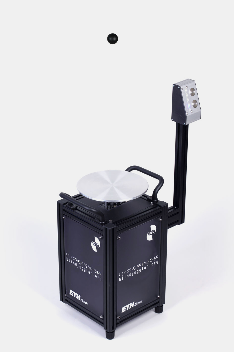
How do you build a robot that can juggle a ball without sensing? In a perfect world, it would not be hard to build: the robot would strike the ball with perfect motion and timing, the ball would be perfectly round, and it would bounce along an ideal path to exactly the same height each time
The world is not perfect, however. Balls that appear round to the eye are actually covered with tiny manufacturing defects, and even the most accurate mechanisms cannot repeat the same motion twice. The result of this imperfect world is that balls do not bounce along a perfect path—they spin, they bounce too high, too low or sideways. In other words, they deviate
Dealing with Deviations
Because the Blind Juggler has no cameras, no microphones or any other sensor to measure the deviations, it cannot actively correct the trajectory of the ball. We must therefore design the robot such that it automatically compensates for the deviations. For example, if the ball bounces up too high, the design has to force the ball to bounce lower again. The goal of the mathematical analysis is to find such a design.
Designing a Stable System
In technical terms, a system that automatically compensates for deviations is called a stable system. We have two parameters at our disposal to stabilize the juggling system: (1) the motion and (2) the shape of the paddle. The goal of the mathematical analysis is to find a stabilizing pair of parameters.
The principle of the analysis is simple: After calculating the ideal trajectory of the ball, we add small deviations to the ideal trajectory. For example, we assume the ball starts off a bit too high, and with some small horizontal velocity. We then use the physical laws of free fall and impact to model how these deviations develop over a series of bounces. If the deviations become smaller with each successive bounce, the system is stable. We therefore search a range of motions and shapes that result in deviations that become smaller over time.
The Key Parameters
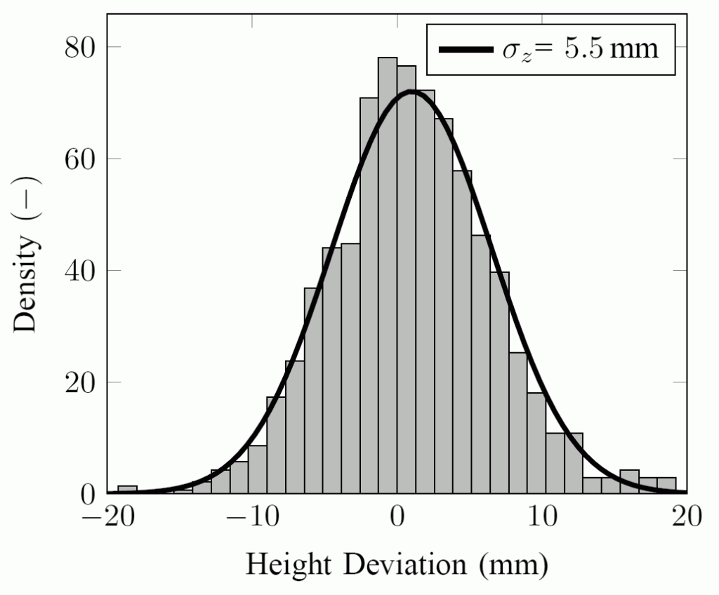
The analysis shows that the paddle must decelerate as it strikes the ball. We can intuitively understand why this makes sense: If the ball bounces too high, it takes longer to return to the paddle; since the paddle is slowing down, the paddle has a lower speed at impact and consequently, the ball bounces less high. The opposite is also true: when the ball is too low, it hits the paddle earlier the next time, so the ball is struck harder and the ball reaches a higher apex again. Therefore, the motion of the paddle forces the ball to maintain a consistent height. On the hardware page, you will find experimental results showing that the ball’s apex height is indeed very consistent.
The Shape
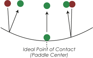
We find that the ball’s trajectory is stabilized in the horizontal directions by a slightly concave
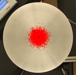
paddle shape. The slight curvature of the paddle keeps the ball in the paddle’s center and prevents the ball from falling off. This is shown in the illustration: The further the ball hits the paddle away from the center, the stronger the ball is pushed inwards again. We find in our analysis that the flatter the plate, the higher we should be able to juggle. We manufactured two paddles: one is a bit flatter than the other one. The prediction our mathematical model makes is indeed true: with the more concave paddle, we can juggle up to about 1.4 meters before the ball falls off; with the flatter paddle, we can go up to 2.0 meters.
Mathematical Background
More specifically, we analyze the dynamics of the deviations. The basic idea of the analysis is quite intuitive when we analyze the following dynamics:![]()
Let ![]() be the impact location deviation of the ball on the paddle, or how far the impact occurs from the paddle center. In the ideal case, this deviation is zero. The parameter
be the impact location deviation of the ball on the paddle, or how far the impact occurs from the paddle center. In the ideal case, this deviation is zero. The parameter ![]() is some number and the index
is some number and the index ![]() denotes the number of the impact. The above equation therefore reads: The impact location at impact
denotes the number of the impact. The above equation therefore reads: The impact location at impact ![]() is
is ![]() times the impact location at impact
times the impact location at impact ![]() . Basically,
. Basically, ![]() describes how the impact location changes between two impacts.
describes how the impact location changes between two impacts.
Now we can think about what this number ![]() has to be such that the ball does not fall off the paddle. Let’s assume that
has to be such that the ball does not fall off the paddle. Let’s assume that ![]() , and that we start with a first impact location of
, and that we start with a first impact location of ![]() . The sequence of impact locations is then
. The sequence of impact locations is then
![Rendered by QuickLaTeX.com \[\begin{aligned}x_1 &= 1 \\x_2 &= 2 x_1 = 2 \times 1 = 2 \\x_3 &= 2 x_2 = 2 \times 2 = 4 \\x_4 &= 2 x_3 = 2 \times 4 = 8 \\\end{aligned}\]](https://blindjuggler.ethz.ch/wp-content/ql-cache/quicklatex.com-06ba6ff9229858c45d158dd3fdfe4102_l3.png)
The impact location doubles at every impact and will get larger and larger. The system is unstable, and the ball will fall off. On the other hand, if ![]() , we get
, we get
![Rendered by QuickLaTeX.com \[\begin{aligned}x_1 &= 1 \\x_2 &= \dfrac{1}{2} x_1 = \dfrac{1}{2} \times 1 = \dfrac{1}{2} \\x_3 &= \dfrac{1}{2} x_2 = \dfrac{1}{2} \times \dfrac{1}{2} = \dfrac{1}{4} \\x_4 &= \dfrac{1}{2} x_3 = \dfrac{1}{2} \times \dfrac{1}{4} = \dfrac{1}{8} \\\end{aligned}\]](https://blindjuggler.ethz.ch/wp-content/ql-cache/quicklatex.com-e5d7d1c9e493daca3029aeac5145c66c_l3.png)
The impact locations get smaller and smaller—the system is stable. The same applies to negative values of ![]() : as long as
: as long as ![]() is between
is between ![]() and
and ![]() , the system is stable. We can therefore conclude that
, the system is stable. We can therefore conclude that ![]() must be in the range
must be in the range
![]()
Nonlinear Systems
An excellent book, which covers the material discussed here in greater detail, is Steven Strogatz’s “Nonlinear Dynamics and Chaos”.
Linear Systems
The linear dynamics we consider on the stability section are
![]()
Think of ![]() as a number describing the dynamical system under analysis, technically referred to as the state of the system. For the Blind Juggler,
as a number describing the dynamical system under analysis, technically referred to as the state of the system. For the Blind Juggler, ![]() could be the impact location of the ball on the paddle. The index
could be the impact location of the ball on the paddle. The index ![]() counts the number of impacts, and
counts the number of impacts, and ![]() is some number, where, for example,
is some number, where, for example, ![]() .
.
The equation then reads: “The impact location ![]() at impact
at impact ![]() is
is ![]() times the location
times the location ![]() at impact
at impact ![]() .” It describes how the impact location changes between two consecutive impacts.
.” It describes how the impact location changes between two consecutive impacts.
Let us analyze the linear dynamics in more detail. First, we find values of ![]() for which a sequence
for which a sequence ![]() remains constant. That means for all
remains constant. That means for all ![]() , the value of
, the value of ![]() does not change. We find that the only
does not change. We find that the only ![]() that fulfills the equation
that fulfills the equation ![]() is
is ![]() .
.
![]()
This specific point where the ![]() remains constant is called a fixed point of the system. We can also find this point by plotting the equation on a graph. Below, we show the linear system dynamics for a range of values of
remains constant is called a fixed point of the system. We can also find this point by plotting the equation on a graph. Below, we show the linear system dynamics for a range of values of ![]() .
.
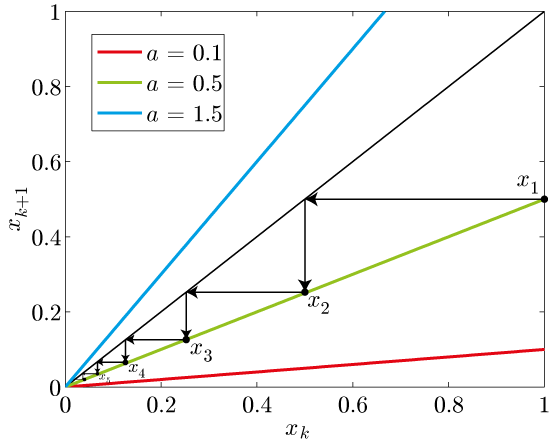
On the lower axis, the impact location at the ![]() -th impact is shown. We can look up what the next impact location is by finding the value of a colored line on the left, vertical axis. Each color corresponds to a different
-th impact is shown. We can look up what the next impact location is by finding the value of a colored line on the left, vertical axis. Each color corresponds to a different ![]() and describes a different dynamical system. The blue line, for example, corresponds to the equation
and describes a different dynamical system. The blue line, for example, corresponds to the equation ![]() . The thin black line is where
. The thin black line is where ![]() . We can use this line to find the fixed point, which is where the black line intersects with the colored line. The intersection is clearly at
. We can use this line to find the fixed point, which is where the black line intersects with the colored line. The intersection is clearly at ![]() for all
for all ![]() .
.
We can also use the black line to visualize how the system evolves over time. Let us see how that works out for the green system dynamics, where ![]() . We start with
. We start with ![]() and find the point on the green line for which
and find the point on the green line for which ![]() . This point is also marked in the figure with
. This point is also marked in the figure with ![]() . To find the next value of
. To find the next value of ![]() , we draw a horizontal arrow from the point
, we draw a horizontal arrow from the point ![]() to the black line, and then add a vertical arrow back to the green line. That gets us to
to the black line, and then add a vertical arrow back to the green line. That gets us to ![]() . Doing this over and over again, we realize that we will approach
. Doing this over and over again, we realize that we will approach ![]() , the fixed point of the system. This is because the fixed point
, the fixed point of the system. This is because the fixed point ![]() is stable for
is stable for ![]() , since
, since ![]() is smaller than one. We discuss this fact in more detail at the end of the stability analysis.
is smaller than one. We discuss this fact in more detail at the end of the stability analysis.
As an aside: set ![]() , and the line describing the system dynamics coincides with the black line. Therefore, any
, and the line describing the system dynamics coincides with the black line. Therefore, any ![]() is a fixed point, and therefore the system has an infinite number of fixed points.
is a fixed point, and therefore the system has an infinite number of fixed points.
Nonlinear Systems
Linear systems are quite straightforward to analyze. To find the fixed point, we need only find the intersection of two straight lines, and we can immediately tell if the fixed point is stable or not by inspecting the parameter ![]() . We will see in a second that this is not straightforward for a nonlinear system.
. We will see in a second that this is not straightforward for a nonlinear system.
As an example, we analyze one of the most famous nonlinear systems, the logistic map. The logistic map can model population growth in biology. You may read more about it here. The system dynamics are
![]()
These dynamics do not look that much more complicated, but they can get very interesting depending on the number you choose for ![]() . This system can be analyzed straightforwardly using the graphical method:
. This system can be analyzed straightforwardly using the graphical method:
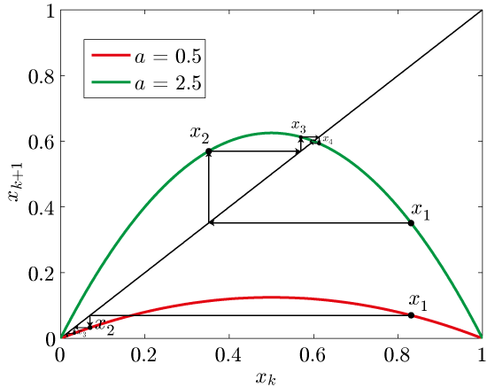
Figure 2: Non linear dynamics
We show the system dynamics for two different values of ![]() . The red system has a fixed point at
. The red system has a fixed point at ![]() , and we find that this fixed point is stable for any starting value we pick in the interval from 0 to 1. The green curve is where things get interesting: If we check the curve for intersections with the black line, we realize that the green system has two fixed points. It intersects at
, and we find that this fixed point is stable for any starting value we pick in the interval from 0 to 1. The green curve is where things get interesting: If we check the curve for intersections with the black line, we realize that the green system has two fixed points. It intersects at ![]() and
and ![]() . Nonlinear systems can have multiple fixed points. The system evolution for the green system, starting at the same value as the red system, shows that the value quickly gets close to the fixed point at 0.6, and then starts spiraling in to the fixed point. Let us have a closer look at this spiraling:
. Nonlinear systems can have multiple fixed points. The system evolution for the green system, starting at the same value as the red system, shows that the value quickly gets close to the fixed point at 0.6, and then starts spiraling in to the fixed point. Let us have a closer look at this spiraling:

Figure 3: Non linear dynamics: spiraling
We see that the red dashed line is actually a pretty good fit to the green line. Therefore, the linear dynamics described by the dashed line are a good approximation to the green, nonlinear system dynamics. For small deviations of ![]() from the fixed point, it is almost perfect. This is exactly how we can analyze the stability of a fixed point of a nonlinear system when deviations are small: We approximate the nonlinear dynamics by linear dynamics, and then analyze these dynamics. This process is called linearization. This is what we did to analyze the stability of the ball motions: We linearized the nonlinear dynamics of the impact locations, assuming the impact locations are small, and then analyzed the resulting linear system dynamics for stability.
from the fixed point, it is almost perfect. This is exactly how we can analyze the stability of a fixed point of a nonlinear system when deviations are small: We approximate the nonlinear dynamics by linear dynamics, and then analyze these dynamics. This process is called linearization. This is what we did to analyze the stability of the ball motions: We linearized the nonlinear dynamics of the impact locations, assuming the impact locations are small, and then analyzed the resulting linear system dynamics for stability.
Back to the example, we find that the approximated system (red, dashed) has the dynamics
![]()
Since ![]() is not smaller than
is not smaller than ![]() , the linear, approximated dynamics are stable (see the stability page why larger than
, the linear, approximated dynamics are stable (see the stability page why larger than ![]() is key). Immediately, we also see why the fixed point at
is key). Immediately, we also see why the fixed point at ![]() of the green system is unstable: The green line is well above the black line. The black line corresponds to linear system dynamics with
of the green system is unstable: The green line is well above the black line. The black line corresponds to linear system dynamics with ![]() , where stable linear systems turn unstable. Therefore, we see that the linearized green system at the
, where stable linear systems turn unstable. Therefore, we see that the linearized green system at the ![]() fixed point has an
fixed point has an ![]() that is larger than
that is larger than ![]() , which indicates that this fixed point is unstable.
, which indicates that this fixed point is unstable.
Periodic Orbits
Now things get even more interesting. We set a = 3.2, and analyze the resulting dynamics:
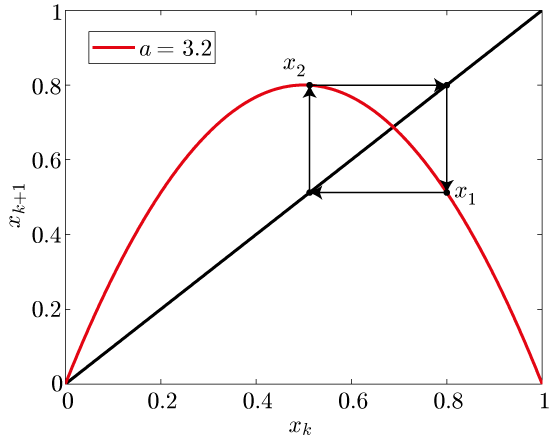
Figure 4: The beauty of periodic orbits.
There are still two fixed points. However, it turns out that if you check their linearized dynamics, both fixed points are unstable. However, we can find another kind of stable system behavior: If we start the system at ![]() ,
, ![]() switches back and forth between 0.8 and 0.51. These two values represent a periodic orbit of the system. We write the following equation for this orbit:
switches back and forth between 0.8 and 0.51. These two values represent a periodic orbit of the system. We write the following equation for this orbit:
![]()
The value of ![]() repeats every other
repeats every other ![]() on this orbit. Therefore, the period of this orbit is two (fixed points are a special class of periodic orbits with period one). Lastly, we find that this periodic orbit is stable: If the system starts near the orbit, it will converge to it, similar to the behavior observed with stable fixed points. With the Blind Juggler, we can also find multiple stable periodic orbits.
on this orbit. Therefore, the period of this orbit is two (fixed points are a special class of periodic orbits with period one). Lastly, we find that this periodic orbit is stable: If the system starts near the orbit, it will converge to it, similar to the behavior observed with stable fixed points. With the Blind Juggler, we can also find multiple stable periodic orbits.
Bifurcation Diagram
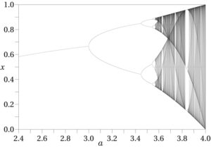
Figure 5: Bifurcation diagram of the logistic map.
For every ![]() , we search the values of
, we search the values of ![]() that are part of a stable periodic orbit of the system. Then, we mark all these points with a black dot. For example, recall the dynamics for
that are part of a stable periodic orbit of the system. Then, we mark all these points with a black dot. For example, recall the dynamics for ![]() , we found a single stable fixed point at
, we found a single stable fixed point at ![]() . Now check the above figure: If you go up from the location on the bottom axis where
. Now check the above figure: If you go up from the location on the bottom axis where ![]() , you will hit the black line exactly at
, you will hit the black line exactly at ![]() . That means that if we increase
. That means that if we increase ![]() from 2.4 to 2.8, the fixed point
from 2.4 to 2.8, the fixed point ![]() also increases, from slightly below 0.6 to about 0.65.
also increases, from slightly below 0.6 to about 0.65.
You can also see that strange things begin to happen as ![]() gets larger. Between 2.4 and 3.0, things are not yet very special; there is only a single stable fixed point. At about 3.0, the fixed point turns into a stable periodic orbit of period two (if you look at the shape of the curve there, it is also clear why this phenomenon is called a bifurcation. At about 3.45, the stable periodic orbit of period two turns into a four-periodic orbit. Further along, we find an 8-periodic orbit, then 16, and so on, until at about 3.6, the system goes completely bananas: it is now chaotic.
gets larger. Between 2.4 and 3.0, things are not yet very special; there is only a single stable fixed point. At about 3.0, the fixed point turns into a stable periodic orbit of period two (if you look at the shape of the curve there, it is also clear why this phenomenon is called a bifurcation. At about 3.45, the stable periodic orbit of period two turns into a four-periodic orbit. Further along, we find an 8-periodic orbit, then 16, and so on, until at about 3.6, the system goes completely bananas: it is now chaotic.
Chaos
A chaotic system has two key properties:
1) Local Instability
The system is locally unstable: If you start the system from two values that are very close to each other, that small difference is amplified and the system quickly evolves very differently for the two starting values (this is illustrated below).
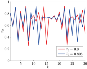
Figure 6: Evolution of the logistic map for ![]() with two close initial conditions.
with two close initial conditions.
The figure shows the system evolution of the logistic map (![]() ) for two starting values that are very close to each other. The blue starting value is just one percent larger than the red starting value, but the system quickly evolves very differently.
) for two starting values that are very close to each other. The blue starting value is just one percent larger than the red starting value, but the system quickly evolves very differently.
2) Strange Attractor
While the system is locally unstable, the system state ![]() does not get arbitrarily large, and remains near a specific set of values called the strange attractor. In the Bifurcation Diagram above, you see that for
does not get arbitrarily large, and remains near a specific set of values called the strange attractor. In the Bifurcation Diagram above, you see that for ![]() , the system won’t take any value
, the system won’t take any value ![]() between 0 and 1 as the system evolves. You will only find values that are black. These black values reveal the strange attractor. It is called an attractor because this black set of values for
between 0 and 1 as the system evolves. You will only find values that are black. These black values reveal the strange attractor. It is called an attractor because this black set of values for ![]() is stable: if the system starts close to this set (for example at
is stable: if the system starts close to this set (for example at ![]() ), it quickly converges to that set of values. This is the same notion of stability as before with the periodic orbits, except that the “stable” motion is now more complicated. The word \emph{strange} in the name stems from the fact that the set of system states
), it quickly converges to that set of values. This is the same notion of stability as before with the periodic orbits, except that the “stable” motion is now more complicated. The word \emph{strange} in the name stems from the fact that the set of system states ![]() that defines the strange attractor is usually not of integer dimension. Such a set could, for example, be neither a line (dimension 1), nor a plane (dimension 2), but something in between. These sets are called fractals.
that defines the strange attractor is usually not of integer dimension. Such a set could, for example, be neither a line (dimension 1), nor a plane (dimension 2), but something in between. These sets are called fractals.
Controllability
Controllability is an important concept in dynamical system theory. For complicated systems with many degrees of freedom and many different control parameters, controllability analysis can tell us whether a system can be controlled to arbitrary configurations from any initial configuration by applying a sequence of control actions. Roughly speaking, the analysis tells us if we have enough ways to influence the system to make it do what we want it to do.
This concept is best explained with a simple toy example. Consider a coin on a plate. The number ![]() describes whether the coin is heads up (
describes whether the coin is heads up (![]() ) or tails up (
) or tails up (![]() ). In dynamical system theory,
). In dynamical system theory, ![]() is called the \emph{state} of the system. We can pick up the coin and turn it to the other side, which is the control parameter we may choose. We can describe the system in the same way as we do in stability analysis and nonlinear systems introduction. The dynamics of the system are
is called the \emph{state} of the system. We can pick up the coin and turn it to the other side, which is the control parameter we may choose. We can describe the system in the same way as we do in stability analysis and nonlinear systems introduction. The dynamics of the system are
![]()
where ![]() is the control action at time
is the control action at time ![]() . At time
. At time ![]() , we can decide whether to turn the coin over or not. Not turning the coin at time
, we can decide whether to turn the coin over or not. Not turning the coin at time ![]() means we choose the control action
means we choose the control action ![]() . This implies that
. This implies that ![]() , and the coin remains unchanged. If we choose
, and the coin remains unchanged. If we choose ![]() , the coin is turned over. For example, suppose the coin is tails up,
, the coin is turned over. For example, suppose the coin is tails up, ![]() , and we choose
, and we choose ![]() . We get
. We get ![]() . The coin is now heads up. In order for the math to make sense, we define that
. The coin is now heads up. In order for the math to make sense, we define that ![]() and
and ![]() , which is the case when we turn the coin from heads to tails:
, which is the case when we turn the coin from heads to tails: ![]() and
and ![]() , so
, so ![]() . This system is controllable. No matter what side of the coin is facing up, we can simply turn it to the side we wish to be facing up.
. This system is controllable. No matter what side of the coin is facing up, we can simply turn it to the side we wish to be facing up.
We can now introduce a system that is similar to juggling multiple balls on a single paddle. Consider two coins on a plate that we can only turn over together. The dynamics are
![Rendered by QuickLaTeX.com \[\begin{cases}x_1(t+1) = x_1(t) + u(t) \mod 2, \\x_2(t+1) = x_2(t) + u(t) \mod 2,\end{cases}\]](https://blindjuggler.ethz.ch/wp-content/ql-cache/quicklatex.com-5aefef3709c9e05125951b39e31b4137_l3.png)
where ![]() and
and ![]() describe the state of the first and second coin at time
describe the state of the first and second coin at time ![]() , respectively. If we choose the control action
, respectively. If we choose the control action ![]() , we flip both coins together. The system is uncontrollable: If the coins start with the same side up, we cannot control them to one coin being heads up and the other tails up, no matter what sequence of control actions we apply.
, we flip both coins together. The system is uncontrollable: If the coins start with the same side up, we cannot control them to one coin being heads up and the other tails up, no matter what sequence of control actions we apply.
Let’s assume we could also choose an additional control action: a simultaneous toss of both coins with a random outcome. If we apply this control, each coin may land heads up or tails up with 50\% probability each. Now the system is controllable in a stochastic (random) sense. Suppose the coins are both face up, and we want to get them to show different sides up. We simply apply the coin toss control action until the coins show different sides. This is a similar strategy to what we use to control multiple balls on the Cloverleaf Blind Juggler into a desired juggling pattern.
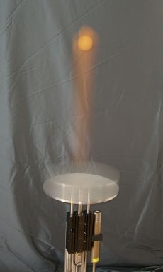
Long exposure shot of first prototype juggling a table tennis ball.
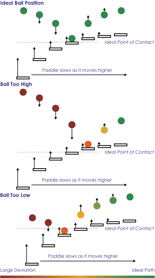
The Motion
Illustration of vertical stability (click to enlarge).
The Shape
Illustration of horizontal stability trough paddle shape.
Impact location data, juggling height 1.05m, 5789 impacts.
Histogram and fitted Gaussian Distribution to apex height deviation data. Juggling height 1.05m, 1079 measurements.
